You have probably heard the word LiDAR more and more over the past few years — in conversations about self-driving cars, drone surveys, autonomous robots, and 3D mapping software. But what exactly is LiDAR, and how does it actually work? This article breaks it all down, step by step, from the moment a laser pulse leaves the sensor to the moment a complete 3D map appears on your screen.
LiDAR is not magic, and it is not complicated once you understand the core principle. At its heart, it asks a very simple question: if I fire a beam of light at something, how long does it take to come back? The answer to that question — measured in billionths of a second — tells us exactly how far away the object is. Do this millions of times per second in every direction, and you build a precise, three-dimensional picture of the entire world around the sensor.
By the end of this article, you will understand every step of that process, the different types of LiDAR systems available today, how LiDAR compares to cameras and radar, and what the final output actually looks like and is used for. If you are planning to build your own LiDAR drone, also check out our complete Low-Cost LiDAR Drone Build Guide at Lidarmos.com — it covers the full hardware and software setup from scratch.
What is LiDAR? The Core Idea
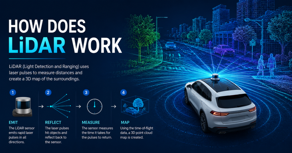
LiDAR stands for Light Detection and Ranging. It is an active remote sensing technology, meaning it generates its own light source rather than relying on the sun or ambient illumination. The sensor fires pulses of laser light — typically in the near-infrared spectrum, invisible to the human eye — and uses a highly sensitive photodetector to catch the light that bounces back.
The fundamental insight that makes LiDAR possible is that light travels at a constant, known speed: approximately 299,792 kilometers per second. This means that if you know exactly when a pulse of light was emitted and exactly when it returned, you can calculate the distance to whatever it bounced off with extraordinary precision.
This technique is called Time-of-Flight, or ToF, and it forms the basis of most LiDAR systems in the world today. The concept is simple. The engineering required to make it work reliably at millions of pulses per second, across hundreds of meters, in rain, dust, and direct sunlight, is considerably more complex — and that engineering is where modern LiDAR startups and sensor manufacturers compete.
Key Concept: LiDAR is essentially a very precise stopwatch attached to a laser. Fire the laser, start the clock. Light returns, stop the clock. Distance = (speed of light x time) / 2.
Step-by-Step: How a LiDAR Pulse Works
The best way to understand LiDAR is to follow a single pulse of light through its entire journey, from the moment it is created to the moment it becomes a data point in a 3D map. The following five steps describe this journey in detail.
Step 1: Emit the Laser Pulse
Inside the LiDAR sensor, a laser diode — similar in principle to the ones found in Blu-ray players, but far more precisely controlled — is triggered by an electronic pulse generator. It emits a burst of infrared light lasting between 2 and 20 nanoseconds. For context, 10 nanoseconds is 0.00000001 seconds. The light is collimated by a small lens so it travels as a narrow, focused beam rather than spreading out immediately.
The laser is typically operating at 905 nanometers wavelength for most commercial sensors, though some longer-range and eye-safe systems use 1550 nm. The pulse is fired at a specific angle determined by the scanning mechanism — more on that in Section 4.
Step 2: Pulse Travels and Hits an Object
The laser pulse travels through air at the speed of light. If there is nothing in its path, it keeps going until it eventually disperses. If it strikes a solid or semi-solid surface — the ground, a building wall, a tree trunk, a vehicle, a person — the light scatters. A portion of that scattered light is reflected back in the general direction of the sensor.
Different materials reflect different amounts of light. Retroreflective surfaces (like road signs or safety vests) reflect strongly and produce a very clear return signal. Dark or absorptive materials (like wet asphalt or black rubber) reflect less light and produce a weaker signal. Modern LiDAR systems are designed to handle this variation in return intensity, and the intensity value of each return is itself recorded as a fourth data channel alongside X, Y, and Z.
Step 3: Return Signal is Detected
The sensor’s receiver — a component called an Avalanche Photodiode (APD) or Single-Photon Avalanche Diode (SPAD) — detects the returning photons. These detectors are extraordinarily sensitive: high-end systems can detect as few as 10 photons returning from a distant surface. The detector converts the incoming photons into an electrical signal, which is then processed by a Time-to-Digital Converter (TDC) — essentially a very precise clock — that records the exact timestamp of the return.
The system compares this return timestamp to the known emission timestamp. The difference between the two is the Time-of-Flight.
Step 4: Distance is Calculated
With the Time-of-Flight value in hand, the onboard processor performs one calculation to determine the distance to the object that reflected the pulse. This is the fundamental LiDAR equation:
Diagram 4: Time-of-Flight Distance Calculation
THE FORMULA:
┌─────────────────────────────────────────────┐
│ │
│ Distance = (c x t) / 2 │
│ │
│ Where: │
│ c = speed of light = 299,792 km/s │
│ t = time of flight (measured in ns) │
│ /2 = divide by 2 (pulse travels TWICE) │
│ │
└─────────────────────────────────────────────┘
WORKED EXAMPLE:
─────────────────────────────────────────────
Pulse emitted at: t = 0.000 ns
Return detected at: t = 65.4 ns
Time of flight (t): 65.4 nanoseconds
Distance = (299,792,458 m/s x 65.4e-9 s) / 2
= (19.606 m) / 2
= 9.80 meters
=> Object is 9.80 meters from the sensor
Diagram 4: Time-of-flight formula with a worked numerical example
The division by two is critical and often confuses beginners: the light travels from the sensor to the target AND back again, so the total distance covered by the light is twice the one-way distance. Dividing by two gives the actual distance to the object.
For a target 9.8 meters away, the time of flight is approximately 65 nanoseconds. For a target at 150 meters — the upper range of many automotive sensors — the time of flight is roughly 1,000 nanoseconds, or 1 microsecond. The precision required to differentiate, say, a 9.80-meter target from a 9.81-meter target requires timing resolution of approximately 0.07 nanoseconds. Modern TDC chips can achieve timing resolution of 10–50 picoseconds (0.01–0.05 nanoseconds), enabling centimeter-level range accuracy.
Step 5: 3D Point is Created and Map is Built
The distance value alone tells us how far something is from the sensor, but not where it is in 3D space. To convert a distance into a 3D coordinate (X, Y, Z), the system also needs to know the exact direction in which the laser was pointing when the pulse was fired. This direction is described by two angles: the horizontal angle (azimuth) and the vertical angle (elevation).
For a drone or vehicle-mounted LiDAR, an additional layer of information is needed: the sensor’s own position and orientation in the world. This is provided by a GPS/GNSS receiver (global position) and an IMU — Inertial Measurement Unit (pitch, roll, and yaw). The combination of range, angles, position, and orientation is sufficient to compute the absolute 3D world coordinates of every single laser return. This is called point cloud georeferencing.
Diagram 1: The Complete LiDAR Pulse Journey
[ LiDAR SENSOR ]
|
| STEP 1: Emit laser pulse (infrared, ~905nm)
| Speed of light: 299,792 km/s
v
~~~~~~~~~~~~~~~~~~~~~~~~~~~~~~~~~~~~>
Laser pulse travels through air
~~~~~~~~~~~~~~~~~~~~~~~~~~~~~~~~~~~~>
|
v
[ TARGET OBJECT ]
(tree / building /
ground / vehicle)
|
| STEP 2: Pulse bounces back
| (reflection / scattering)
v
<~~~~~~~~~~~~~~~~~~~~~~~~~~~~~~~~~~~~
Return signal travels back
<~~~~~~~~~~~~~~~~~~~~~~~~~~~~~~~~~~~~
|
v
[ DETECTOR / RECEIVER ]
|
| STEP 3: Measure Time-of-Flight (ToF)
| t = time between emit and return
v
[ COMPUTE ] Distance = (Speed of Light x t) / 2
|
| STEP 4: Combine with scan angle + GPS
v
[ 3D POINT ] X, Y, Z coordinates
|
| Repeat millions of times per second
v
[ POINT CLOUD ] Full 3D map of environment
Diagram 1: Step-by-step path of a single LiDAR laser pulse — from emission to 3D map point
Repeat this process for every pulse the sensor fires — which can be anywhere from 100,000 to 2.4 million times per second — and over the course of a flight or drive, tens or hundreds of millions of 3D points accumulate to form a dense, accurate representation of the entire scanned environment.
Diagram 2: How Individual Points Build a 3D Map
SINGLE PULSE => 1 data point
——————————–
Pulse #1 => Point (x:0.0, y:0.0, z:2.4m)
Pulse #2 => Point (x:0.1, y:0.0, z:2.4m)
Pulse #3 => Point (x:0.2, y:0.0, z:2.4m)
… => …
Pulse #1M => Point (x:5.0, y:5.0, z:0.0m)
RESULT after 1,000,000 pulses:
. . . . . . . . . . <- Rooftop
. . <- Wall face
. . . . . . . . . . <- Window ledge
. . <- Wall
. . . . . . . . . . . <- Ground
* * * * * * * * * * * <- Shadow returns
Each dot = 1 laser return = 1 3D coordinate
Density: 100 pts/m2 (low) to 2000 pts/m2 (high)
Diagram 2: Accumulation of millions of laser returns to form a dense 3D point cloud
Key Technical Specifications
Now that you understand the core process, here is a reference table of the key technical parameters used to describe and compare LiDAR sensors:
| Parameter | Typical Values / Range |
| Laser Wavelength | 905 nm (most sensors) | 1550 nm (eye-safe, longer range) |
| Pulse Rate | 100,000 – 2,400,000 pulses per second (Hz) |
| Range | 5 m (indoor robots) to 300 m (automotive sensors) |
| Accuracy | 1 – 5 cm typical | sub-1 cm with RTK GPS correction |
| Field of View | Single-point (1°) to 360° horizontal + 45° vertical |
| Point Density | 10 pts/m² (low-altitude slow scan) to 2,000 pts/m² (dense) |
| Operating Temp | -40°C to +85°C (automotive grade) |
| Power Consumption | 3W (LD06 small sensor) to 60W (Velodyne VLP-32C) |
| Data Output Format | LAS / LAZ (GIS) | PCD (ROS) | PLY (3D visualization) |
Table 1: Key LiDAR technical parameters and typical values across different sensor classes
How LiDAR Sensors Scan: The Mechanics
A single laser pointed in one fixed direction would only measure one distance — the distance to whatever is directly in front of it. Useful LiDAR systems need to scan in multiple directions simultaneously or in rapid sequence to build a 3D picture of the environment. Several different scanning technologies are used to achieve this.
Mechanical Spinning LiDAR
The original and still most common design for high-performance LiDAR is the mechanical spinning sensor. A cluster of laser emitters and detectors is mounted on a rotating platform that spins 360 degrees continuously, typically at 10–20 rotations per second. Each emitter covers a vertical slice of the world, and together they cover the full hemisphere.
The Velodyne HDL-32E and VLP-16 are classic examples of this design. They contain 32 or 16 laser emitters stacked vertically, each angled at a different elevation, and the entire assembly spins to provide a 360-degree horizontal field of view. The result is a cylindrical point cloud around the sensor, with vertical resolution determined by the number of laser channels.
Solid-State LiDAR (MEMS)
Mechanical spinning sensors are reliable and high-performance, but they contain moving parts that can wear out, are relatively large and heavy, and are expensive to manufacture. Solid-state LiDAR replaces the rotating platform with MEMS (Micro-Electro-Mechanical Systems) mirrors — microscopic silicon mirrors that tilt back and forth thousands of times per second to steer the laser beam across the scene without any large-scale mechanical motion.
MEMS LiDAR sensors are smaller, lighter, and cheaper to manufacture than spinning sensors, making them practical for consumer automotive ADAS (Advanced Driver Assistance Systems) applications. The tradeoff is typically a smaller field of view — a MEMS sensor might cover 120 degrees horizontal rather than 360 degrees.
Flash LiDAR
Flash LiDAR takes a completely different approach: instead of scanning a beam across the scene, it illuminates the entire field of view at once with a single wide laser flash — similar to how a camera flash works. A 2D array of photodetectors captures the return from every point in the scene simultaneously, producing an instant 3D depth image without any scanning motion.
Flash LiDAR is very fast — it can capture full-scene depth images at video frame rates — but current technology limits its practical range to roughly 30–50 meters, making it suitable for close-range robotics and gesture recognition rather than long-range mapping.
FMCW LiDAR
FMCW (Frequency Modulated Continuous Wave) is a fundamentally different approach that is gaining significant commercial traction. Rather than measuring the time of flight of a discrete pulse, FMCW LiDAR continuously emits a beam whose frequency changes over time, and measures the frequency difference between the emitted and returned light. This frequency shift encodes not just distance but also the Doppler velocity of the target — its speed relative to the sensor.
FMCW LiDAR delivers instant velocity measurement for every point in the scene simultaneously, without additional processing. As described in our Top LiDAR Startups 2025 article at Lidarmos.com, this is the technology that Aeva Technologies has commercialized and is deploying with major automotive OEMs. FMCW is also inherently immune to interference from other LiDAR sensors — a critical advantage as autonomous vehicles become more common on public roads.
Diagram 5: Complete LiDAR System Components ┌──────────────────────────────────────────┐
│ LIDAR SYSTEM OVERVIEW │
├───────────────┬──────────────────────────┤
│ TRANSMITTER │ RECEIVER │
│ ● Laser diode│ ● Photodetector (APD) │
│ ● Pulse gen │ ● TDC (time-to-digital) │
│ ● Collimator │ ● Signal amplifier │
├───────────────┴──────────────────────────┤
│ SCANNING MECHANISM │
│ ● Rotating mirror (mechanical) │
│ ● MEMS micro-mirror (solid state) │
│ ● Flash LiDAR (no moving parts) │
├──────────────────────────────────────────┤
│ POSITIONING (for drones / vehicles) │
│ ● GPS / GNSS (global position) │
│ ● IMU (pitch, roll, yaw) │
│ ● RTK GPS (cm-level accuracy) │
├──────────────────────────────────────────┤
│ COMPUTE & OUTPUT │
│ ● Onboard FPGA / processor │
│ ● Point cloud generation │
│ ● SLAM / mapping algorithms │
│ ● Export: LAS / LAZ / PLY / PCD │
└──────────────────────────────────────────┘
Diagram 5: Internal architecture of a complete LiDAR system — from laser to point cloud output
Types of LiDAR Sensors: A Complete Comparison
With the scanning mechanisms understood, here is a complete comparison of the main LiDAR sensor types available today:
| Type | Example | How It Works | Pros | Cons | Best For |
| Mechanical / Spinning | Velodyne HDL-32 | Rotating motor spins 360° | High density, proven | Bulky, moving parts | Automotive survey |
| Solid-State (MEMS) | Innoviz One | Micro-mirrors, no rotation | Compact, durable | Smaller FOV | ADAS, robotics |
| Flash LiDAR | Aeye iDAR | Full scene illuminated at once | Fast frame rate | Short range | Close-range robotics |
| FMCW | Aeva Atlas | Continuous frequency wave | Instant velocity | Complex hardware | Autonomous trucks |
| Single-Point | Garmin LIDAR-Lite | One beam only | Cheap, simple | No mapping use | Altitude hold, ranging |
| 2D Scanning | RPLIDAR A1 | Horizontal plane scan | Low cost (~$99) | 2D only | Indoor robots, DIY drones |
Table 2: LiDAR sensor type comparison — technology, use cases, pros and cons
LiDAR vs. Cameras vs. Radar
LiDAR is not the only sensor technology available for autonomous systems and mapping applications. Cameras and radar each have distinct capabilities and limitations. Understanding how LiDAR compares to these alternatives is essential for understanding why it is used and when.
| Feature | LiDAR | Camera (RGB) | Radar |
| 3D Depth Data | Yes — direct measurement | Requires stereo / computation | Yes — but low resolution |
| Works in Darkness | Yes — active sensor | No — needs ambient light | Yes — active sensor |
| Works in Rain / Fog | Partially | Poor | Yes — best performer |
| Point Density | High (millions/sec) | N/A (pixels, not points) | Low (tens of points) |
| Range Accuracy | 2–5 cm typical | 5–50 cm (stereo) | 10–50 cm |
| Color / Texture | No | Yes — full color | No |
| Detects Velocity | Only FMCW type (Aeva) | Via optical flow | Yes — Doppler native |
| Cost (entry level) | $30 – $500 | $5 – $100 | $200 – $2,000 |
| Best Use Case | 3D mapping, obstacle avoidance | Object classification, color | Speed detection, weather |
Table 3: Sensor technology comparison — LiDAR vs. RGB camera vs. radar
In practice, autonomous vehicles and high-end robotics systems rarely rely on a single sensor type. A typical autonomous car sensor suite includes LiDAR (for precise 3D mapping), multiple cameras (for color, texture, and object classification), and radar (for velocity detection and weather resilience). The combination is called sensor fusion, and it is the industry standard approach to building robust, redundant perception systems.
Why Not Just Use Cameras? Cameras are cheap and provide rich color information, but they cannot directly measure distance — they only see the world in 2D. Computing 3D depth from cameras requires either stereo setups (two cameras) or complex neural networks, both of which introduce latency and error. LiDAR provides direct, instantaneous 3D measurement.
How LiDAR Works on a Drone
When LiDAR is mounted on a drone rather than a ground vehicle or fixed tripod, the workflow has several additional steps and considerations. This is the most relevant configuration for surveying, mapping, agriculture, and inspection applications.
The Drone-Mounted LiDAR Workflow
Diagram 3: LiDAR Drone Scanning a Site from Above
DRONE IN FLIGHT (altitude: 50-100m AGL)
==========================================
[DRONE]
|
LiDAR Spins 360deg
/ | \
/ | \
v v v
. . . <- Scan lines hit ground
SIDE VIEW (showing scan fan below drone):
[DRONE]—-(GPS+IMU records position)
/ | | | \
/ | | | \ <- LiDAR scan fan
/ | | | \ (FOV ~360 deg)
v v v v v
. . . . . . . . . . . <- Ground returns
GGGGGGGGGGGGGGGGGGGGG <- Ground surface
Drone speed: 5-8 m/s | Overlap: 80% frontlap
Point density: 50-200 pts/m2 at 60m altitude
Diagram 3: LiDAR drone scanning pattern — sensor rotates 360 degrees as drone moves forward
- Mission planning: The drone’s flight path is programmed as a grid pattern over the target area, with altitude, speed, and overlap settings chosen to achieve the desired point density.
- Pre-flight setup: GPS is acquired, the IMU is calibrated, and the LiDAR sensor is powered on and verified. The RTK GPS base station is deployed if centimeter-level accuracy is needed.
- Flight and scanning: As the drone follows the programmed grid, the LiDAR sensor rotates continuously, firing hundreds of thousands of pulses per second. GPS and IMU data are recorded synchronously with every laser return.
- Data download: After landing, the raw point cloud data (LAS or binary format), GPS trajectories, and IMU logs are downloaded to a processing computer.
- Post-processing: Specialized software (CloudCompare, LiDAR360, Terrasolid) merges the GPS trajectory with the point cloud, applies IMU corrections for sensor orientation, and produces a fully georeferenced 3D map.
- Output products: The processed data is used to generate Digital Elevation Models (DEMs), contour maps, volumetric calculations, 3D building models, or vegetation height maps depending on the application.
The Role of the IMU
The IMU deserves special attention because it is critical to data quality in airborne LiDAR. A drone in flight is never perfectly level or perfectly still — it pitches, rolls, and yaws constantly in response to wind gusts and control inputs. If these movements are not corrected in the data, a slight 2-degree roll that occurs during a scan will shift all the points recorded at that moment by several meters, creating errors in the final map.
The IMU records these orientation changes at high frequency (typically 200–400 Hz), and post-processing software uses this data to mathematically “un-rotate” each point back to its true position. High-quality IMU integration is one of the biggest differences between professional and consumer-grade LiDAR drone systems.
What Does LiDAR Data Look Like? Point Clouds Explained
The output of a LiDAR scan is a point cloud — a collection of millions of individual 3D coordinates, each representing a location where a laser pulse returned. Visualizing a point cloud for the first time is often a striking experience: complex environments like forests, city blocks, or building interiors appear as dense, ghostly clouds of colored dots that together form a recognizable 3D shape.
Point Cloud Data Attributes
- X, Y, Z coordinates: The 3D position of each return in a defined coordinate system (e.g., WGS84 for global, or a local projected system)
- Intensity: The strength of the return signal (0–255 scale), which reflects surface reflectivity and material properties
- Return number: LiDAR pulses can produce multiple returns from a single shot — e.g., through gaps in a tree canopy, a pulse might return once from the leaves and again from the ground below
- Point time: The timestamp of each return, enabling time-series analysis and trajectory correction
- RGB color (if camera co-registered): Optional color values added by fusing with a simultaneous RGB camera image
Point Cloud File Formats
- LAS (.las): Industry standard format from the American Society for Photogrammetry and Remote Sensing (ASPRS); stores all standard LiDAR attributes
- LAZ (.laz): Compressed version of LAS; typically 5–10x smaller file size with no data loss
- PCD (.pcd): ROS (Robot Operating System) native format; widely used in robotics applications
- PLY (.ply): Common in 3D visualization and graphics pipelines
- E57 (.e57): Used for terrestrial laser scanner data; supports structured scan formats
From Point Cloud to Useful Products
Raw point clouds are rarely the final product. They are processed further to extract specific information:
- Digital Terrain Model (DTM) / Digital Elevation Model (DEM): A raster grid of ground elevation values, used in hydrology, land management, and construction
- Digital Surface Model (DSM): Includes the tops of all objects (buildings, trees) rather than bare ground
- Contour maps: Lines of equal elevation, generated from the DEM for engineering and surveying
- Vegetation height model (CHM): DSM minus DTM = height of vegetation above ground, used in forestry
- Building footprints and 3D city models: Automated extraction of building shapes for urban planning and BIM
- Volume calculations: Cut/fill analysis for earthworks, stockpile measurement for mining and construction
Real-World Applications of LiDAR
The combination of precision, speed, and automation that LiDAR enables makes it relevant across an extraordinarily wide range of industries.
Autonomous Vehicles
This is the application that brought LiDAR into mainstream awareness. Autonomous cars and trucks use LiDAR to build a real-time 3D model of the road environment, detecting other vehicles, pedestrians, cyclists, road boundaries, and obstacles at ranges of up to 200 meters. The sensor’s ability to work in complete darkness and its direct 3D depth output make it a critical complement to camera-based perception systems.
Aerial Surveying and Mapping
Drone-mounted and aircraft-mounted LiDAR systems are used by surveying companies, government agencies, and utility operators to create highly accurate terrain models and infrastructure maps. Applications include flood risk modeling, corridor mapping for power lines and pipelines, archaeological site detection through vegetation, and topographic survey for construction projects.
Agriculture
In precision agriculture, LiDAR enables crop canopy analysis, terrain modeling for irrigation planning, and autonomous guidance for farm machinery. As described in our article on the top LiDAR startups to watch in 2025 (Lidarmos.com), companies like Agtonomy are retrofitting existing farm equipment with LiDAR systems to automate routine tasks on vineyards and row-crop farms.
Construction and Infrastructure
LiDAR is used throughout the construction lifecycle: from initial site survey and earthwork planning, through BIM model validation during construction, to as-built documentation on completion. The ability to quickly and accurately compare a point cloud of the as-built structure against the original design model is transforming quality control on major projects.
Mining and Hazardous Environment Inspection
As covered in our startups article, companies like Exyn Technologies use AI-powered drones with LiDAR to inspect underground mines and collapsed structures — environments where sending human workers poses serious safety risks. The drone builds a 3D map autonomously without GPS, using SLAM (Simultaneous Localization and Mapping) algorithms.
Forestry and Environmental Monitoring
Airborne LiDAR is the gold standard tool for forest inventory and biomass estimation. By measuring the height and density of tree canopies from aircraft or drones, LiDAR enables ecologists to assess carbon stocks, track deforestation, model wildlife habitat, and monitor post-fire recovery across large areas — tasks that would be impossible at scale with ground-based methods.
Common Misconceptions About LiDAR
As LiDAR becomes more widely discussed, several misconceptions frequently appear. Here are the most important ones to address:
- LiDAR and radar are the same thing: No. Radar uses radio waves and excels in weather and velocity detection but has very low spatial resolution. LiDAR uses laser light and provides centimeter-accurate 3D spatial data. They are complementary technologies, not alternatives.
- LiDAR cannot work in sunlight: Incorrect. Modern LiDAR sensors are designed to operate in full sunlight. They use narrow bandpass optical filters to reject ambient light and only admit wavelengths matching the sensor’s laser. Solar interference was a problem with early sensors but has been effectively solved in sensors manufactured since 2015.
- LiDAR works by taking photos: LiDAR does not capture images. It measures distances. The colorized point cloud visualizations you may have seen online are created by fusing LiDAR distance data with color information from a separate RGB camera — the color does not come from the LiDAR itself.
- One LiDAR sensor is enough for full autonomy: Autonomous systems require redundancy and complementary perception. A camera can recognize a stop sign; LiDAR knows exactly how far away it is. Radar can detect a vehicle in fog; LiDAR can map the road surface. These sensors work best together.
- LiDAR is only useful at close range: Entry-level sensors have ranges of 12–40 meters, but mid-range automotive sensors reach 150–250 meters, and airborne survey sensors commonly operate at altitudes of 500–2000 meters above ground.
Conclusion
LiDAR is a elegant technology built on a simple physical principle: light travels at a constant speed, so measuring how long a pulse takes to return tells you exactly how far it traveled. Scaled up to millions of pulses per second, combined with precise positioning and orientation data, and processed by modern software, this simple principle becomes one of the most powerful sensing technologies ever developed for mapping, navigation, and automation.
Understanding LiDAR at the level described in this article — from the physics of a single pulse, through the mechanics of scanning, to the georeferencing of millions of returns into a 3D map — gives you the foundation to evaluate LiDAR systems, understand their limitations, and apply them intelligently to real problems.
If you are interested in building your own LiDAR drone system, our complete Low-Cost LiDAR Drone Build Guide at Lidarmos.com walks you through every component, wiring step, and software setup needed to get from parts to flying in a budget of $500 to $1,500. And if you want to understand which companies are pushing the boundaries of LiDAR technology in 2025, our Top LiDAR Startups article profiles five companies — Aeva, Exyn, Nuro, Outrider, and Agtonomy — with real funding data and technical analysis.

